Unexpected molecular sexual dimorphisms (in host-microbial interactions).
While wandering through the literature, I found myself reading a paper by departmental colleagues Dong Tian, Mingxue Cui, and Min Han (2024). They describe effects of bacterial mucopolysaccharides, components of bacterial cell walls, on mitochondrial functions in mice and human cells. While an interesting example of the interaction between components of the microbiome and its host, what was particularly surprising to me was their observation that these mucopolysaccharides had sex-specific effects on mitochondrial functions (footnote 1). This sexual dimorphism was documented by examining the generation of reactive oxygen species (ROS) formed during reactions involving molecular oxygen (O2), concentrations of ATP (cells’ primary energy currency), and body weight, when comparing control mice with mice treated with “an antibiotic cocktail to deplete the intestinal microbiota in order to eliminate the source of muropeptides following a well-established protocol for antibiotic-induced microbiome depletion (AIMD)”. One interesting result was that the addition of bacteria-derived proteoglycan derived “muropeptides” (see their figure 3 ↓ (modified) and the included image, derived from it with scale modifications) dramatically inhibited the effects of AIMD treatment on a number of cellular behaviors in mouse and human cells.
Perhaps It should be expected that removing an organism’s internal microbiome causes a number of stress effects on the host, nor that mitochondria (derived, via endosymbiosis and subsequent evolutionary adaptations) respond to such changes. Mitochondrial functions seem particularly sensitive to general cellular stresses (a topic considered in more detail in the appearance of mitochondrial stress effects associated with “knock-out” mutations in a number of intermediate filament proteins (the work of others reviewed here).
What was surprising (certainly to me) was the observation that male and female cells responded differently to muropeptides; something reported previously by Gabanyi et al (2022). There are, of course, a number of possible and plausible reasons for such differences. For one, a recent study of the cellular (gene-protein) network involved in male gamete formation further revealed its evolutionarily ancient origin and its complexity, involving the “expression of approximately 10,000 protein-coding genes, a third of which define a genetic scaffold of deeply conserved genes” (Brattig-Correia et al., 2024). While this study focussed on the male germ lines, the tissue that generates sperm, it is likely that differences in gene expression occur throughout the body. As an example, based on analyses of protein expression in post-mortem human brain tissues Wingo et al (2023) reported that “Among the 1,239 proteins, 51% had higher expression in females and 49% had higher expression in males”.
In this light, It is tempting to speculate that the effects of mucoproteins might well extend beyond the mouse and lead to sex-specific differences in humans as well. The source of these differences could be the result of cellular and tissue specific differences sex-influenced variations in gene expression, protein activity, and cellular organization, including social interactions between cells in tissues and organs. They may arise as indirect (and complex) effects of androgen or estrogen-based hormone responses. It is interesting how these differences may or may not impact a range of physiological effects.
It might seem a stretch to claim that experimental observations on how mice navigate a maze in the dark, in a laboratory can provide meaningful and actionable insights into how to improve the design of undergraduate science courses, but that is my claim. They provide a parable about what matters in education.
If I correctly understand the implications of the work from Markus Meister’s lab (Rosenberg et al 2021. Mice in a labyrinth: Rapid learning, sudden insight, and efficient exploration) one take home message is that mice learn remarkably quickly if the tasks they are presented with “make sense” to them, that the task reflects something they would be expected to master naturally. A dark maze mimics such a case, the exploration of an underground burrow system. Within this system they are challenged to find water (when thirsty) and their way home when they decide to go home. In these studies, the mice were tracked in the absence of human intervention; the mice were free to stay in their cages, or enter and explore the maze – and explore it they did, completely and efficiently. This reflects their spontaneous behavior. In other cases, the mice were mildly deprived of water. They quickly found a water source located within the maze and learned to remember its location. Even more striking, the mice were extremely efficient at finding their way back home (navigating their way out of the maze) when they wanted to, making few miss turns. They rapidly mastered these tasks and the progression in their mastery was often characterized by what might be termed a “eureka moment”, a point when their behavior becomes significantly more goal oriented and efficient.
The efficiency of their maze learning compares to what appears to be slow, tedious and ineffective learning of what are known as “two-alternative-forced-choice (2AFC)” tasks, tasks that can take months for mice to “master” ineffectively. These are “un-mouse-like” tasks that appear to be of little intrinsic interest to the average mouse.
It is difficult (at least for me) not to see an analogy with educational situations, although a number of factors combine to make humans students rather less homogenous than inbred lines of laboratory mice. Nevertheless, and since this is a parable rather than a logical extension of the Rosenberg et al study, we can speculate that students will be better at engaging with and mastering tasks that are seen as natural and interesting compared to tasks that they judge to be artificial, irrelevant, and in some cases threatening (e.g. exams). At the same time, we can see the importance of the eureka moment, the point at which a key insight into a task becomes apparent. Of course it is worth placing Archimedes’ eureka moment in context – after all
he had been asked to solve an important problem by Hieron, the king of Syracuse. The solution came to him while he was engaged in an activity (taking a bath) that displays the relevant physical principle, buoyancy, the key insight needed to solve the problem.
There are a number of lessons here. Perhaps the first is that exploring and patrolling underground burrows (the maze) and exploring the universe (science) are not so different – they can both be ‘naturally’ engaging tasks. But too often science (or rather courses in science, particularly required courses, come across as chores, to be completed. Their relevance to the students’ interests and goals may be unclear; in a well designed curriculum, their relevance is made obvious. But these are also not ordinary chores, they are “graded chores”. One wonders whether mice “punished ” for inadequate maze behavior might eventually choose to stop exploring mazes (or underground burrows).
Then there is the organization of the maze, does it reflect a real problem faced by mice, or is it an artificial task, meant to sort rather than teach? Does learning the maze help with other problems to be faced. Does the task focus on core and widely applicable principles or idiosyncratic features. Does the task lose sight of what matters? These are questions that can be applied at many points within the process of course design and delivery – when is memorization important (and there are times it can be useful) and when is it a distraction, often evidence of lazy course design. When is it important to let the student explore, encourage questions, provide useful, and perhaps more importantly provocative, socratic feedback that students are required to address, and either incorporate into their thinking or explain why it is irrelevant. My own conclusion from the parable of the mouse and the maze is to be mindful of what you want students to be able to do when you introduce facts, principles and tasks. Question the value of introducing details that could be deduced from over-arching principles, and don’t introduce material that you do not intend to have students apply. Avoid google-able insights.
Perhaps a real life biology laboratory example may be useful. When asked to generate a solution with a specific pH do you, as a sophisticated lab rat, sit down and calculate the amounts of all of the various compounds needed to produce that pH, or do you use a pH meter and titrate the solution? While there are situations where calculations are useful, for many (most) situations the pH meter approach makes more sense (assuming of course you can explain why it works, e.g. what amount of chemical you begin with, and whether you should add an acid or a base to produce the desired pH).
A lesson for instructors is that it is important to present science in the context of a coherent and compelling narrative, a narrative that provides an understanding of the implications and significance of the information presented, so that the answer actually matters to the student. This is a process that involves reconsidering content, and it can be difficult to disconnect from what and how you were taught. It requires that you, as the instructor, come to recognize ideas and principles you use when “doing science”. When you discover a dramatic disconnect from what you present to students and what you use when you confront a problem, it is time to redesign your course to make it a more interesting (and rewarding) maze.
If there is one thing that university faculty and administrators could do today to demonstrate their commitment to inclusion, not to mention teaching and learning over sorting and status, it would be to ban curve-based, norm-referenced grading. Many obstacles exist to the effective inclusion and success of students from underrepresented (and underserved) groups in science and related programs. Students and faculty often, and often correctly, perceive large introductory classes as “weed out” courses preferentially impacting underrepresented students. In the life sciences, many of these courses are “out-of-major” requirements, in which students find themselves taught with relatively little regard to the course’s relevance to bio-medical careers and interests. Often such out-of-major requirements spring not from a thoughtful decision by faculty as to their necessity, but because they are prerequisites for post-graduation admission to medical or graduate school. “In-major” instructors may not even explicitly incorporate or depend upon the materials taught in these out-0f-major courses – rare is the undergraduate molecular biology degree program that actually calls on students to use calculus or a working knowledge of physics, despite the fact that such skills may be relevant in certain biological contexts – see Magnetofiction – A Reader’s Guide. At the same time, those teaching “out of major” courses may overlook the fact that many (and sometimes most) of their students are non-chemistry, non-physics, and/or non-math majors. The result is that those teaching such classes fail to offer a doorway into the subject matter to any but those already comfortable with it. But reconsidering the design and relevance of these courses is no simple matter. Banning grading on a curve, on the other hand, can be implemented overnight (and by fiat if necessary).
So why ban grading on a curve? First and foremost, it would put faculty and institutions on record as valuing student learning outcomes (perhaps the best measure of effective teaching) over the sorting of students into easy-to-judge groups. Second, there simply is no pedagogical justification for curved grading, with the possible exception of providing a kludgy fix to correct for poorly designed examinations and courses. There are more than enough opportunities to sort students based on their motivation, talent, ambition, “grit,” and through the opportunities they seek after and successfully embraced (e.g., through volunteerism, internships, and independent study projects).
The negative impact of curving can be seen in a recent paper by Harris et al, (Reducing achievement gaps in undergraduate general chemistry …), who report a significant difference in overall student inclusion and subsequent success based on a small grade difference between a C, which allows a student to proceed with their studies (generally as successfully as those with higher grades) and a C-minus, which requires them to retake the course before proceeding (often driving them out of the major). Because Harris et al., analyzed curved courses, a subset of students cannot escape these effects. And poor grades disproportionately impact underrepresented and underserved groups – they say explicitly “you do not belong” rather than “how can I help you learn”.
Often naysayers disparage efforts to improve course design as “dumbing down” the course, rather than improving it. In many ways this is a situation analogous to blaming patients for getting sick or not responding to treatment, rather than conducting an objective analysis of the efficacy of the treatment. If medical practitioners had maintained this attitude, we would still be bleeding patients and accepting that more than a third are fated to die, rather than seeking effective treatments tailored to patients’ actual diseases – the basis of evidence-based medicine. We would have failed to develop antibiotics and vaccines – indeed, we would never have sought them out. Curving grades implies that course design and delivery are already optimal, and the fate of students is predetermined because only a percentage can possibly learn the material. It is, in an important sense, complacent quackery.
Banning grading on a curve, and labelling it for what it is – educational malpractice – would also change the dynamics of the classroom and might even foster an appreciation that a good teacher is one with the highest percentage of successful students, e.g. those who are retained in a degree program and graduate in a timely manner (hopefully within four years). Of course, such an alternative evaluation of teaching would reflect a department’s commitment to construct and deliver the most engaging, relevant, and effective educational program. Institutional resources might even be used to help departments generate more objective, instructor-independent evaluations of learning outcomes, in part to replace the current practice of student-based opinion surveys, which are often little more than measures of popularity. We might even see a revolution in which departments compete with one another to maximize student inclusion, retention, and outcomes (perhaps even to the extent of applying pressure on the design and delivery of “out of major” required courses offered by other departments).
“All a pipe dream” you might say, but the available data demonstrates that resources spent on rethinking course design, including engagement and relevance, can have significant effects on grades, retention, time to degree, and graduation rates. At the risk of being labeled as self-promoting, I offer the following to illustrate the possibilities: working with Melanie Cooper at Michigan State University, we have built such courses in general and organic chemistry and documented their impact, see Evaluating the extent of a large-scale transformation in gateway science courses.
Perhaps we should be encouraging students to seek out legal representation to hold institutions (and instructors) accountable for detrimental practices, such as grading on a curve. There might even come a time when professors and departments would find it prudent to purchase malpractice insurance if they insist on retaining and charging students for ineffective educational strategies.(1)
Acknowledgements: Thanks to daughter Rebecca who provided edits and legal references and Melanie Cooper who inspired the idea. Educate! image from theDorian De Long Arts & Music Scholarship site.
(1) One cannot help but wonder if such conduct could ever rise to the level of fraud. See, e.g., Bristol Bay Productions, LLC vs. Lampack, 312 P.3d 1155, 1160 (Colo. 2013) (“We have typically stated that a plaintiff seeking to prevail on a fraud claim must establish five elements: (1) that the defendant made a false representation of a material fact; (2) that the one making the representation knew it was false; (3) that the person to whom the representation was made was ignorant of the falsity; (4) that the representation was made with the intention that it be acted upon; and (5) that the reliance resulted in damage to the plaintiff.”).
A RAG-ChatGPT written backgrounder (checked and edited by Mike Klymkowsky ) for the excessively curious – in support of biofundamentals – 1 August 2025
Weldon’s Background and Perspective: Walter F. R. Weldon (1860–1906) was a British zoologist and a pioneer of biometry – the statistical study of biological variation. He believed that evolution operated through numerous small, continuous variations rather than abrupt, either-or traits. In his studies of creatures like shrimps and crabs, Weldon found that even traits which appeared dimorphic at first could grade into one another when large enough samples were measured [link]. He and his colleague Karl Pearson (1857-1936) argued that Darwin’s theory of natural selection was best tested with quantitative methods: “the questions raised by the Darwinian hypothesis are purely statistical, and the statistical method is the only one at present obvious by which that hypothesis can be experimentally checked” [link]. This emphasis on gradual variation and statistical analysis set Weldon at odds with the emerging Mendelian school of genetics, led by William Bateson (1861-1926) that focused on discrete traits and sudden changes. By 1902, the scientific community had split into two camps – the biometricians (Weldon and Pearson in London) versus the Mendelians (Bateson and allies in Cambridge) – reflecting deep disagreements over the nature of heredity [link]. This was the charged backdrop against which Weldon evaluated Gregor Mendel’s pea-breeding experiments.
Critique of Mendel’s Pea Traits and CategoriesWeldon’s photographic plate of peas illustrating continuous variation in seed color. (This figure from his 1902 paper shows pea seeds ranging from green to yellow in a smooth gradient, contradicting the clear-cut “green vs. yellow” categories assumed by Mendel [link]. Images 1–6 and 7–12 (top rows) display the range of cotyledon colors in two different pea varieties after the seed coats were removed [link]. Instead of all seeds being simply green or yellow, Weldon documented many intermediate shades. He even found seeds whose two cotyledons (halves) differed in color, underscoring that Mendel’s binary categories were oversimplifications of a more complex reality [link].
Weldon closely re-examined the seven pea traits Mendel had chosen (such as seed color and seed shape) and argued that Mendel’s tidy classifications did not reflect biological reality in peas. In Mendel’s account, peas were either “green” or “yellow” and produced either “round, smooth” or “wrinkled” seeds, with nothing in between. Weldon showed this was an artifact of Mendel’s experimental design. He gathered peas from diverse sources and found continuous variation rather than strict binary types. For example, a supposedly pure “round-seeded” variety produced seeds with varying degrees of roundness and wrinkling [link]. Likewise, seeds that would be classified as “green” or “yellow” in Mendel’s scheme actually exhibited a spectrum of color tones from deep green through greenish-yellow to bright yellow [link]. Weldon’s observations were impossible to reconcile with a simple either/or trait definition [link].
Weldon concluded that Mendel had deliberately picked atypical pea strains with stark, discontinuous traits, and that Mendel’s category labels (e.g. “green vs. yellow” seeds) obscured the true, much more variable nature of those characters [link]. In Weldon’s view, the neat ratios Mendel obtained were only achievable because Mendel worked with artificially generated lines of peas, bred to eliminate intermediate forms [link]. In ordinary pea populations that a farmer or naturalist might encounter, such clear-cut divisions virtually disappeared: “Many races of peas are exceedingly variable, both in colour and in shape,” Weldon noted, “so that both the category ‘round and smooth’ and the category ‘wrinkled and irregular’ include a considerable range of varieties.” [link] In short, he felt Mendel’s chosen traits were too simple and unrepresentative. The crisp binary traits in Mendel’s experiments were the exception, not the rule, in nature. Weldon’s extensive survey of pea varieties led him to believe that Mendel’s results “had no validity beyond the artificially “purified”in-bred” races Mendel worked with,” because the binary categories “obscured a far more variable reality.”[link]
Mendel’s Conclusions and Real-World Heredity. Weldon went beyond critiquing Mendel’s choice of traits – he questioned whether Mendel’s conclusions about heredity were biologically meaningful for understanding inheritance in real populations. Based on his empirical findings and evolutionary perspective, Weldon doubted that Mendel’s laws could serve as general laws of heredity. Some of his major biological objections were:
–Traits are seldom purely binary in nature: Outside the monk’s garden, most characteristics do not sort into a few discrete classes. Instead, they form continuous gradations. Weldon realized that Mendel’s insistence on traits segregating neatly into “either/or” categories “simply wasn’t true,” even for peas [link]. Mendel’s clear ratios were achieved by excluding the normal range of variation; in the wild, peas varied continuously from yellow to green with every shade in between [link]. What Mendel presented as unitary “characters” were, in Weldon’s eyes, extremes picked from a continuum.
– Mendel’s results were an artifact of pure-breeding: Weldon argued that the famous 3:1 ratios and other patterns were only apparent because Mendel had used highly inbred, “pure” varieties. By extensive inbreeding and selection, Mendel stripped away intermediate variants [link]. The artificially uniform parent strains used in Mendel’s experiments do not reflect natural populations. Weldon concluded that the seeming universality of Mendel’s laws was misleading – they described those special pea strains, not peas (or other organisms) at large [link]. In a letter, he even mused whether Mendel’s remarkably clean data were “too good” to be true, hinting that real-world data would rarely align so perfectly [link].
– Dominance is not an absolute property: A cornerstone of Mendelism was that one trait form is dominant over the other (e.g. yellow dominates green). Weldon questioned this simplistic view. He gathered evidence that whether a given trait appears dominant or recessive can depend on context – on the plant’s overall genetic background and environmental conditions [link]. For example, a seed color might behave as dominant in one cross but not in another, if other genetic factors differ. Weldon argued that Mendel’s concept of dominance was “oversimplified” because it treated dominance as inherent to a trait, independent of development or ancestry [link]. In reality (as Weldon emphasized), “the effect of the same bit of chromosome can be different depending on the hereditary background and the wider environmental conditions”, so an inherited character’s expression isn’t fixed as purely dominant or recessive [link]. This questioned the biological generality of Mendel’s one-size-fits-all dominance rule.
– Atavism and ancestral influence: Perhaps most intriguing was Weldon’s concern with reversion (atavism) – cases where an offspring exhibits a trait of a distant ancestor that had seemingly disappeared in intervening generations. Breeders of plants and animals had long reported that occasionally a “throwback” individual would appear, showing an old parental form or color after many generations of absence. To Weldon, such phenomena implied that heredity isn’t solely about the immediate parents’ genes, but can be influenced by more remote ancestral contributions [link]. “Mendel treats such characters as if the condition in two given parents determined the condition in all their offspring,” Weldon wrote, but breeders know that “the condition of an organism does not as a rule depend upon [any one pair of ancestors] alone, but in varying degrees upon the condition of all its ancestors in every past generation” [link]. In other words, the influence of a trait could accumulate or skip generations. This idea directly conflicted with Mendel’s theory as presented in 1900, which only considered inheritance from the two parents and had no mechanism for latent ancestral traits resurfacing after several generations. Weldon concluded from examples of reversion that Mendel’s framework was biologically incomplete – there had to be “more going on” in heredity than Mendel’s laws acknowledged [link].
In sum, Weldon found Mendel’s laws too limited and idealized to account for the messy realities of inheritance in natural populations. Mendel had demonstrated elegant numerical ratios with a few pea characters, but Weldon did not believe those results scaled up to the complex heredity of most traits or species. Variation, continuity, and context were central in Weldon’s view of biology, whereas Mendel’s work (as interpreted by Mendel’s supporters) seemed to ignore those factors. Thus, Weldon saw Mendel’s conclusions as at best a special case – interesting, but not the whole story of heredity in the real world [link][link].
Weldon’s Legacy
Weldon’s critiques came at a time of intense debate between the “Mendelians” and the “Biometricians.” William Bateson, the chief Mendelian, vehemently defended Mendel’s theory against Weldon’s attacks. In 1902, Bateson published a lengthy rebuttal titled Mendel’s Principles of Heredity: A Defense, including a 100-page polemic aimed squarely at “defending Mendel from Professor Weldon”[link]. Bateson and his allies believed Weldon had misinterpreted Mendel and that discrete Mendelian factors really were the key to heredity. The clash between Weldon and Bateson grew increasingly personal and public. By 1904 the feud had become so heated that the editor of Nature refused to publish any further exchanges between the two sides [link]. At a 1904 British Association meeting, a debate between Bateson and Weldon on evolution and heredity became a shouting match, emblematic of how divisive the issue had become [link][link].
Although Weldon’s objections were rooted in biological observations, many contemporaries saw the dispute as one of old guard vs. new ideas. Tragically, Weldon died in 1906 at the age of 46, with a major manuscript on inheritance still unfinished [link]. In that unpublished work, he had gathered experimental data to support a more nuanced theory reconciling heredity with development and ancestral effects [link][link]. With his early death, much of Weldon’s larger critique faded from the spotlight. Mendelian genetics, championed by Bateson and later enriched by the chromosome theory, surged ahead. Nevertheless, in hindsight many of Weldon’s points were remarkably prescient. His insistence on looking at population-level variation and the importance of multiple factors and environment foreshadowed the modern understanding that Mendelian genes can interact in complex ways (for example, polygenic inheritance and gene-by-environment effects). As one historian noted, Weldon’s critiques of Mendelian principles were “100 years ahead of his time” [link]. In the context of his era, Weldon doubted the biological relevance of Mendel’s peas for the broader canvas of life – and while Mendel’s laws did prove fundamental, Weldon was correct that real-world heredity is more intricate than simple pea traits. His challenge to Mendelism ultimately pushed geneticists to grapple with continuous variation and population dynamics, helping lay the groundwork for the synthesis of Mendelian genetics with biometry in the decades after his death[link][link].
Sources: Weldon’s 1902 paper in Biometrika and historical analyses [link][link][link][link][link][link][link]provide the basis for the above summary. These document Weldon’s arguments that Mendel’s pea traits were overly simplistic and his laws of heredity not universally applicable to natural populations, especially in light of continuous variation, context-dependent trait expression, and atavistic reversions. The debate between Weldon and the Mendelians is detailed in contemporary accounts and later historical reviews [link][link], illustrating the scientific and conceptual rift that formed around Mendel’s rediscovered work.
background: I have long been interested in students’ (and the public’s) misconceptions about biology (see this & that). More and more, it appears to me that part of the problem arises when conventional biology (and science courses in general) leave underlying scientific principles unrecognized and/or unexplained. In biology, there is a understandable temptation to present processes in simple unambiguous ways, often by ignoring the intrinsic complexity and underlying molecular scale of these systems. The result is widespread confusion among the public, a confusion often exploited by various social “influencers”, some (rather depressingly) currently in positions of power within the US.
After attending a recent Ray Troll and Kirk Johnson roadshow on fossils, art, and public engagement at the Denver Museum of Nature and Science (DMNS), I got to thinking. As a new hobby, in advance of retirement, perhaps I can work on evolving the tone of my writing to become less “academical” and more impactful, engaging, and entertaining (at least to some) while staying scientifically accurate and comprehensible. So here goes an attempt (helped out by genAI).
A common misconception, promoted by some “science popularizers” is that biological systems, including humans, are “determined” or “super-determined” (what ever that means) by various factors, particularly by the versions of genes, known as alleles, they inherited from their parents. While there is no question that biological systems are influenced and constrained by a number of factors (critical to “stay’n alive), the idea of determinism seems problematic (considered here). So where would a belief in biological determinism come from? One possibility, that emerged in the “Teaching and Learning Biology” course taught with Will Lindsay@CU Boulder, is the way basic genetics is often presented to students. The specific topic that caught my attention was the way the outcome of genetic crosses (matings) was presented, specifically through the use of what are known as Punnett’s squares.
In a typical sexually reproducing organism, the parents with different mating types or sexes, e.g. male and female, have two copies of each gene (mostly) – they are termed “diploid”. The two versions of a particular gene can be the same, in which case the organism is said to be “homozygous” or different, when it is termed “heterozygous” for that gene. The allele(s) carried by one parent can be the same or different from the allele(s) carried by the other. Molecular analysis of the alleles present in a population has been key to determining who, back in the day, was mating with Neanderthals (see wikipedia). Each gamete (egg or sperm) produced contains one or the other version of each gene – they are termed “haploid”. When sperm and egg fuse, a new diploid organism is generated.
Much of what is described above was figured out by Gregor Mendel (wikipedia). The good monk employed a few tricks that enabled him to recognize (deduce) key genetic “rules”. First, he worked with peas, Pisum sativum and related species. He used plants grown by commercial plant breeders to have specific versions of a particular trait. In his studies, he focussed on plants that displayed versions of traits that were unambiguously distinguishable from one another. Such pairs of traits are termed dichotomous; they exist in one or the other unambiguously recognizable form, without overlapping intermediates. The majority of traits are continuous rather than dichotomous.
As part of the process of generating “predictable plants”, breeders select male and female plants with the traits that they seek and discard others. After many generations the result are plants with reproducible and predictable traits. Does this mean that the plants are identical? Nope! There is still variability between individual plants of the same “strain”. For example, Mendel used strains of “tall” and “short” pea plants; the tall plants had stem lengths of between ~6 to 7 feet while the short plants had stem lengths between ~0.75 to 1.5 feet (a two-fold variation)(see Curtis, 2023). He put them into tall and short classes, ignoring these differences. But these plants were different. Such differences arise through stochastic processes and responses to developmental and environmental effects that impact height in various ways (discussed in a past post). Mendel began his studies with 22 strains of pea plants but only 7 exhibited the dichotomous behaviors he wanted. If he had included the others, it is likely he would have been confused and never would have arrived at his clean genetic rules. In fact, after he published his studies on peas, he took the advice of Carl Nägeli (see wikipedia) and began studies using Hieracium (hawkweeds), which differs in its reproductive strategy from Pisum (Nogler 2006). Nägeli’s suggestion and Mendel studies lead to uncertainty about the universality of Mendel’s rules. Mendel’s experiences reflect a key feature of scientific studies: simplify, get interpretable data, and then extend observations / systems leading to confirmation or revision.
The variation inherent in biological systems is nicely illustrated by what is (or should be) a classic study by Vogt et al (2008) who described the variations that occur within populations of genetically identical shrimp raised in identical conditions. The variation between genetically similar organisms (or identical twins) found in the wild (natural populations) is much greater. Why? because in breeder supplied plants most of the allelic variation present in the wild population is lost, discarded in the process of selecting and breeding organisms for specific traits. We see these “genetic background” effects when looking at genetically determined traits in humans as well. Consider cystic fibrous, a human genetic disease associated with the inheritance of altered versions of the CFTR gene (more on cystic fibrosis). People who inherit two disease-associated alleles of the CFTR gene develop cystic fibrosis, but as noted by Corvol et al (2015) “patients who have the same variants in CFTR exhibit substantial variation in the severity of lung disease” and this variation is associated (explained by) genetic background effects, together with stochastic effects and their developmental and environmental histories. In any of a number of studies, whenever populations of organisms are analyzed based on their genotype (which alleles they carry) the result is inevitably a distribution of responses, even when the average responses are different (for a good example see Löscher 2024).
In the case of the traits Mendel studied, he concluded that the trait was determined by the presence of different versions (alleles) of a genetic “factor”, that each organism contained two alleles, that these alleles could be the same (homozygous) or different (heterozygous), and that one allele was “dominant” to the other (“recessive”). If the dominant allele were present, it would determine the form of the trait observed. Only if both versions of the alleles present were recessive would the organism display the associated trait. The other rule was that all of the gametes produced by homozygous organism carried the same “trait-producing” allele, while heterozygous organisms produced gametes containing one or the other allele.
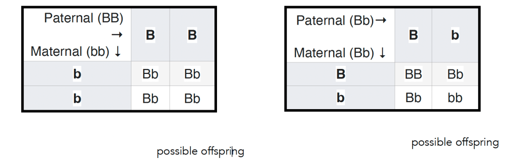
In 1905 Reginald Punnett introduced a way of thinking about Mendel’s matings, a diagram now known as a Punnett’s square (see wikipedia). In this figure (left below) ↓ the outcome of a mating between a male homozygous for a dominant allele and a female homozygous for a recessive allele is illustrated. All of the offspring will be heterozygous, but it is worth keeping in mind, however, that does not mean that they will be identical – they will display a similar level of variation in the trait seen in populations of the parental plants (see above). Again, this variation arises from the impact of environmental effects on developmental processes together with the influence of stochastic effects. The variation associated with the particular set of alleles present in an organism is captured by what is known as variable penetrance and expressivity of a gene-influenced trait (see link for molecular details). Ignoring the variations observed between organisms carrying the same allele(s) of a gene (or the same genotype in identical twins or clones can encourage or reinforce the idea that the details of an organism (its phenotype) are determined by the alleles it carries.
Another way students’ belief in genetic determinism can be reinforced is perhaps unintentional. Typically the result of the original mating between homozygous recessive and dominant parents (the P generation) is termed the first filial or F1 generation. Often the next type of genetic cross presented to students involves crossing male and female F1 individuals to produce the second filial or F2 generation (see figure – right above ↑). Such as F1 cross is predicted to produce organisms that display the dominant to recessive trait in a ratio of 3 to 1. What is often missing is that reproducible observation of this ratio requires that large numbers of F2 organisms are examined. The result of any particular F1 (heterozygous) cross is unpredictable; it can vary anywhere from 0 to 4 dominant to recessive trait displaying organisms to 4 to 0 trait dominant to recessive trait displaying organisms, and anything in between. This behavior is characteristic of a stochastic process; predictable when large numbers of events are considered and unpredictable when small numbers of events are considered. Stochastic behaviors are common in biological organisms, given the small numbers of particular molecules, and specifically particular genes, they contain (a GoldLabSymposium talk on the topic). In the context of organisms, there is room for something like “free will” (consideredhere). Whether Elon “knows” he is giving something that closely resembles a Nazi salute or not, we can presume that he is, at least partially, responsible for his actions and by implication their ramifications.
Why are the results of a mating stochastic? Because which gamete contains which trait-associated allele occurs by chance, while which gametes fuse together to produce the embryo is again a chance event. Some analyses of the numbers Mendel originally reported led to suggestions that his numbers were “too good”, and the perhaps he fudged them (for a good summary see Radick 2022). The bottom line – subsequent studies have repeatedly confirmed Mendel’s conclusions with the important caution that the link between genotype and phenotype is typically complex and does not obey strictly deterministic rules.
Nota bene: This is not mean to be a lesson in genetics; if interested in going deeper I would recommend you read Jamieson & Radick (2013) and the genetics section of biofundamentals.
Literature cited:
Corvol et al., (2015). Genome-wide association meta-analysis identifies five modifier loci of lung disease severity in cystic fibrosis. Nature communications, 6, 8382.
Curtis (2023). Mendel did not study common, naturally occurring phenotypes. Journal of Genetics, 102(2), 48.
Jamieson & Radick (2013). Putting Mendel in his place: How curriculum reform in genetics and counterfactual history of science can work together. In The philosophy of biology: A companion for educators (pp. 577-595). Dordrecht: Springer Netherlands.
Löscher (2024). Of Mice and Men: The Inter-individual Variability of the Brain’s Response to Drugs. Eneuro, 11(2).
Nogler (2006). The lesser-known Mendel: his experiments on Hieracium. Genetics, 172(1), 1-6.
Radick (2022). Mendel the fraud? A social history of truth in genetics. Studies in History and Philosophy of Science, 93, 39-46.
van Heyningen (2024). Stochasticity in genetics and gene regulation. Philosophical Transactions of the Royal Society B, 379(1900), 20230476.
Cells are extremely complex.1 Much of their “core” complexity appears to have been present in their last (universal) common ancestor, known as LUCA. We find it in the “conserved” molecular mechanisms and machines active in modern cells. LUCA and its offspring are membrane-bounded, non-equilibrium systems that import free energy and export entropy to maintain and repair themselves, to grow, behave, and reproduce (and all the other things living things do). One problem, however, with LUCA is that it makes speculation on the steps that preceded it impossible to know with certainty. Not withstanding claims of breakthroughs (e.g. ‘Monumental’ experiment suggests how life on Earth may have started“), it is likely that we will never know the actual steps involved; after all, the origin of life occurred billions of years ago and under rather different conditions than exist today.
Living systems “work” based on inherited, pre-existing molecular machines and mechanisms (1). The actions of these machines are fueled through coupling to thermodynamically favorable reactions taking place under non-equilibrium conditions, i.e. the living state. Looking at the details of these interactions reveals interesting and unexpected behaviors. Unfortunately, the “simple” physical-chemical underpinnings of these processes, key to understanding them, are not always presented to students effectively (2). At the same time, the complexity of cellular systems means that in practice, the link between “simple” molecular mechanisms and the behavior of a biological systems can be obscure (see 3). That said, key insights are illuminated when molecular mechanisms are examined, as illustrated by Wee et al., (2023)(4).
Emerging from LUCA, biological populations have diverged into distinct “prokaryotic” lineages: the bacteria and archaea.2 Both are defined by a protein-lipid boundary layer, the plasma membrane. Within this membrane is a single internal compartment, the cytoplasm. Information is stored in cells in two forms, first in the on-going LUCA-derived living system and the second, information in the sequence of double-stranded DNA molecules. These two types of information are interdependent: the information in DNA makes sense only within a cell and the on-going cellular processes depend upon and utilize the information in DNA. In bacteria and archaea, these are circular double-stranded DNA molecules. Here we restrict our discussion to the common unicellular bacterium Escherichia coli (E. coli), one of the workhorse systems that led to an understanding of core molecular mechanisms.
E. coli hasa single circular genomic DNA molecule of ~5 million nucleotide base pairs in length; it contains about 5000 distinct genes that encode polypeptides and functional “non-coding” RNA molecules (if you are interested in numbers, check out bionumbers). An E. coli cell is rod-shaped and ~1 micrometer (10-6 meters) long. Its genomic DNA molecule is ~1000 times longer than the cell that contains it, and a rapidly dividing cell can contain multiple copies of the genome. Genes typically contain two distinct functional regions. Regulatory regions interact with various proteins that determine whether a gene is “expressed” or not. Coding regions specify what is expressed. The first step is the synthesis of an RNA molecule; such a molecule can encode a polypeptide or a non-coding RNA.3 Non-coding RNAs can have structural, catalytic, or regulatory functions.
The first step in gene expression in all cell types is the binding of proteins to a gene’s regulatory sequences. Typically a complex of proteins leads to the binding and activation of a DNA-dependent, RNA polymerase. The RNA polymerase complex unwinds a specific region of the DNA and uses the complementary nature of nucleotide base pairing: A binding to T in DNA and U in RNA, and C binding to G in both, to synthesize an RNA molecule based on DNA sequence. Synthesis of RNAs that encode polypeptides, known as messenger RNAs (mRNAs) starts with the 5′ end of the molecule and moves toward the 3′ end (replaced ↓ soon).
In prokaryotic cells, both DNA and mRNA synthesis reactions occur in the cytoplasm. A ribosome, a molecular machine composed of multiple proteins and RNAs, can engage the 5′ end region of an mRNA as soon as it appears – before the synthesis of the mRNA is complete. The cytoplasm of a cell contains lots of ribosomes; in E. coli there are ~70,000 ribosomes per cell (more or less). This leads to some interesting and functionally significant interactions. One thing to consider, not always stressed, is that these synthetic processes are not error proof. DNA replication (DNA-directed, DNA synthesis), transcription (DNA-directed, RNA synthesis), and polypeptide synthesis (RNA-directed, polypeptide synthesis) all have an error rate, typically 1 error per ~106 addition events for DNA replication and transcription. Errors can lead to mutations in the DNA, RNAs that encode abnormal proteins, or abnormal and potentially toxic polypeptides.
To deal with physical realities, these synthetic processes employ various “error correction” strategies. In the case of DNA and RNA synthesis, the polymerases involved have what is known as “proof-reading” activities. If the incorrect nucleotide is inserted into a growing DNA or RNA chain, it can be recognized; the polymerase can then “reverse” (move backward along the DNA), remove the mistakenly inserted nucleotide, and then move forward again, adding the correct nucleotide. Key here is that the polymerase is moving back and forth along the DNA strand. The result of proof-reading is to reduce the error rate of DNA-dependent DNA and RNA synthesis substantially, down to 10-8 to 10-10 per base pair in the case of DNA synthesis.
In the case of the RNA polymerase, the newly synthesized RNA can fold back on itself, forming what is known as a “hairpin”. This hairpin “can stabilize an elemental pause (in RNA synthesis) an allosteric interaction with the β-flap tip helix of RNAP”. What Wee et al (4) report is as the mRNA-associated ribosome moves along the RNA it unfold the hairpin and “bumps” into the polymerase, inhibiting this “pause” which increases the rate of mRNA synthesis and inhibits the polymerase’s error correction function. The resulting mRNA population has more frequent base pair changes, errors that can influence the polypeptides synthesized. While cells of all types have various “chaperone” systems that can deal with misfolded proteins that arise in response to various stresses or errors, these can be overwhelmed. The resulting misfolded (damaged) proteins can lead to cellular defects and long term effects on viability (discussed in 5).
About 1.5 billion years later (give or take), a new type of cell appeared, the result (apparently) of a symbiotic interaction between an archaeal-like “host” and a O2-utilizing bacterium. This synthetic organism, the progenitor of the eukaryotes, differed from either type of prokaryote in that it sequestered its genome, now composed of linear DNA molecules, within a double membrane bounded “nuclear” compartment. In this hybrid cell type, DNA and RNA synthesis was confined to the nucleus, while ribosomes and polypeptide synthesis were confined to the cytoplasm. Eukaryotic cells are typically much larger that prokaryotic cells, reproduce more slowly, and are more complex in terms of the numbers of genes, and the amount of genomic DNA they contain. It is tempting to speculated that while rapidly dividing, relatively simple prokaryotic cells may be able to tolerate more mistakes in terms of the synthesis of their polypeptides, larger, more complex eukaryotic cells would be vulnerable. A plausible result would be a selection pressure to separating RNA from polypeptide synthesis.
literature cited
Alberts, B. (1998). The cell as a collection of protein machines: preparing the next generation of molecular biologists. Cell, 92, 291-294.
de Lorenzo, V., 2024. The principle of uncertainty in biology: Will machine learning/artificial intelligence lead to the end of mechanistic studies?. Plos Biology, 22, p.e3002495.
Image from Govindjee – doi:10.3389/fpls.2011.00028, CC BY 3.0. Given the diversity of biological systems, these are general descriptions – often there a exceptions, but recognizing them all makes generating a coherent narrative difficult (and beyond me). Mea culpa. ↩︎
You might be constrained and contingent on past events, but you are not determined! (that said you are not exactly free either).
AI Generated Summary: Arguments for and against determinism and free will in relation to biological systems often overlook the fact that neither is entirely consistent with our understanding of how these systems function. The presence of stochastic, or seemingly random, events is widespread in biological systems and can have significant functional effects. These stochastic processes lead to a range of unpredictable but often useful behaviors. When combined with self-consciousness, such as in humans, these behaviors are not entirely determined but are still influenced by the molecular and cellular nature of living systems. They may feel like free actions, but they are constrained by the inherent biological processes.
Recently two new books have appeared arguing for (1) and against (2) determinism in the context of biological systems. There have also been many posts on the subject (here is the latest one by John Horgan. These works join an almost constant stream of largely unfounded, and bordering on anti-scientific speculation, including suggestions that consciousness has non-biological roots and exists outside of animals. Speaking as a simple molecular/cellular biologist with a more than passing interest in how to teach scientific thinking effectively, it seems necessary to anchor any meaningful discussion of determinism vs free will in clearly defined terms. Just to start, what does it mean to talk about a system as “determined” if we can not accurately predict its behavior? This brings us to a discussion of what are known as stochastic processes.
The term random is often use to describe noise, unpredictable variations in measurements or the behavior of a system. Common understanding of the term random implies that noise is without a discernible cause. But the underlying assumption of the sciences, I have been led to believe, is that the Universe is governed exclusively by natural processes; magical or supernatural processes are not necessary and are excluded from scientific explanations. The implication of this naturalistic assumption is that all events have a cause, although the cause(s) may be theoretically or practically unknowable. For example, there are the implications of Heisenberg’s uncertainty principle, which limits our ability to measure all aspects of a system. On the practical side, measuring the position and kinetic energy of each molecule (and the parts of larger molecules) in a biological system is likely to kill the cell. The apparent conclusion is that the measurement accuracy needed to consider a system, particularly a biological system as “determined” is impossible to achieve. In a strict sense, determinism is an illusion.
The question that remains is how to conceptualize the “random”and noisy aspects of systems. I would argue that the observable reality of stochasticity, particularly in biological systems at all levels of organization, from single cells to nervous systems, largely resolves the scientific paradox of randomness. Simply put, stochastic processes display a strange and counter-intuitive behavior: they are unpredictable at the level of individual events, but the behaviors of populations become increasingly predictable as population size increases. Perhaps the most widely known examples of stochastic processes are radioactive decay and Brownian motion. Given a large enough population of atoms, it is possible to accurately predict the time it takes for half of the atoms to decay. But knowing the half-life of an isotope does not enable us to predict when any particular atom will decay. In Schrödinger’s famous scenario a living cat is placed in an opaque box containing a radioactive atom; when the atom decays, it activates a process that leads to the death of the cat. At any particular time after the box is closed, it is impossible to predict with certainty whether the cat is alive or dead because radioactive decay is a stochastic process. Only by opening the box can we know for sure the state of the cat. We can, if we know the half-life of the isotope, estimate the probability that the cat is alive but rest assured, as a biologist who has a cat, at no time is the cat both alive and dead. We cannot know the “state of the cat” for sure until we open the box.
Something similar is going on with Brownian motion, the jiggling of pollen grains in water first described by Robert Brown in 1827. Einstein reasoned that “if tiny but visible particles were suspended in a liquid, the invisible atoms in the liquid would bombard the suspended particles and cause them to jiggle”. His conclusion was that Brownian motion provided evidence for the atomic and molecular nature of matter. Collisions with neighboring molecules provides the energy that drives diffusion; it drives the movement of molecules so that regulatory interactions can occur and provides the energy needed to disrupt such molecular interactions. The stronger the binding interaction between atoms or molecules the longer, ON AVERAGE, they will remain associated with one another. We can measure interaction affinities based on the half-life of interactions in a large enough population, but as with radioactive decay when exactly any particular complex dissociates cannot be predicted.
Molecular processes clearly “obey” rules. Energy is moved around through collisions, but we cannot predict when any particular event will occur. Gene expression is controlled by the assembly and disassembly of multicomponent complexes. The result is that we cannot know for sure how long a particular gene will be active or repressed. The result of such unpredictable assembly/disassembly events leads to what is known as transcriptional bursting; bursts of messenger RNA synthesis from a gene followed by periods of “silence” (3). A similar behavior is associated with the synthesis of polypeptides (4). Both processes can influence cellular and organismic behaviors. Many aspects of biological systems, including embryonic development, immune system regulation, and the organization and activity of neurons and supporting cells involved in behavioral responses to external and internal signals (5), display such noisy behaviors.
Why are biological systems so influenced by stochastic processes? Two simple reasons – they are composed of small, sometimes very small numbers of specific molecules. The obvious and universal extreme is that a cell typically contains one to two copies of each gene. Remember, a single change in a single gene can produce a lethal effect on the cell or organism that carries it. Whether a gene is “expressed” or not can alter, sometimes dramatically, cellular and system behaviors. The number of regulatory, structural, and catalytic molecules (typically proteins) present in a cell is often small leading to a situation in which the effects of large numbers do not apply. Consider a “simple” yeast cell. Using a range of techniques Ho et al (6) estimated that such cells contain about 42 million protein molecules. A yeast cell has around 5300 genes that encode protein components, with an average of 8400 copies of each protein. In the case of proteins present at low levels, the effects of noise can be functionally significant. While human cells are larger and contain more genes (~25,000) each gene remains at one to two copies per cell. In particular, the number of gene regulatory proteins tends to be on the low side. If you are curious the B10NUMB3R5 site hosted by Harvard University provides empirically derived estimates of the average number of various molecules in various organisms and cell types.
The result is that noisy behaviors in living systems are ubiquitous and their effects unavoidable. Uncontrolled they could lead to the death of the cell and organism. Given that each biological system appears to have an uninterrupted billion year long history going back to the “last universal common ancestor”, it is clear that highly effective feedback systems monitor and adjust the living state, enabling it to respond to molecular and cellular level noise as well as various internal and external inputs. This “internal model” of the living state is continuously updated to (mostly) constrain stochastic effects (7).
Organisms exploit stochastic noise in various ways. It can be used to produce multiple, and unpredictable behaviors from a single genome, and are one reason that identical twins are not perfectly identical (8). Unicellular organisms take advantage of stochastic processes to probe (ask questions of) their environment, and respond to opportunities and challenges. In a population of bacteria it is common to find that certain cells withdraw from active cell division, a stochastic decision that renders them resistant to antibiotics that kill rapidly dividing cells. These “persisters” are no different genetically from their antibiotic-sensitive relatives (9). Their presence enables the population to anticipate and survive environmental challenges. Another unicellular stochastically-regulated system is the bacteria E. coli‘s lac operon, a classic system that appears to have traumatized many a biology student. It enables the cell to ask “is there lactose in my environment?” How? A repressor molecule, LacI, is present in about 10 copies per cell. When more easily digestible sugars are absent the cell enters a stress state. In this state, when the LacI protein is knocked off the gene’s regulatory region there is a burst of gene expression. If lactose is present the proteins encoded by the operon are synthesized and enable lactose to enter and be broken down. One of the breakdown products inhibits the repressor protein, so that the operon remains active. No lactose present? The repressor rebinds and the gene goes silent (10). Such noisy regulatory processes enables cells to periodically check their environment so that genes stay on only when they are useful.
As noted by Honegger & de Bivort (11)(see also post on noise) decades of inbreeding with rodents in shared environments eliminated only 20–30% of the observed variance in a number of phenotypes. Such unpredictability can be beneficial. If an organism always “jumps” in the same direction on the approach of a predator it won’t take long before predators anticipate their behavior. Recent molecular techniques, particularly the ability to analyze the expression of genes at the single cell level, have revealed the noisiness of gene expression within cells of the same “type”. Surprisingly, in about 10% of human genes, only the maternal or the paternal version of a gene is expressed in a particular cell, leading to regions of the body with effectively different genomes. This process of “monoallelic expression” is distinct from the dosage compensation associated with the random “inactivation” of one or the other X-chromosomes in females. Monoallelic expression has been linked to “adaptive signaling processes, and genes linked to age-related diseases such as neurodegeneration and cancer” (12). The end result of noisy gene expression, mutation, and various “downstream” effects is that we are all mosaics, composed of clones of cells that behave differently due to noisy molecular differences.
Consider your brain. On top of the recently described identification of over 3000 neural cell types in the human brain (13), there is noisy as well as experience-dependent variation in gene expression, neuronal morphology and connectedness, and in the rates and patterns of neuronal firing due to differences in synaptic structure, position, strength, and other factors. Together these can be expected to influence how you (your brain) perceives and processes the external world, your own internal state, and the effects associated with the interaction between these two “models”. Of course the current state of your brain has been influenced, constrained by and contingent upon by past inputs and experiences, and the noisy events associated with its development. At the cellular level, the sum of these molecular and cellular interactions can be considered the consciousness of the cell, but this is a consciousness not necessarily aware of itself. In my admittedly naive view, as neural systems, brains, grow in complexity, they become aware of their own workings. As Godfrey-Smith (14) puts it, “brain processes are not causes of thoughts and experiences; they are thoughts and experiences”. Thoughts become inputs into the brain’s model of itself.
What seems plausible is that as nervous systems increase in complexity, processing increasing amounts of information including information arising from its internal workings, it may come to produce a meta-model that for reasons “known” only to itself needs to make sense of those experiences, feelings, and thoughts. In contrast to the simpler questions asked by bacteria, such as “is there an antibiotic or lactose in my world?”, more complex (neural) systems may ask “who is to blame for the pain and suffering in the world?” I absent-mindedly respond with a smile to a person at a coffeehouse, and then my model reconsiders (updates) itself depending, in part, upon their response, previous commitments or chores, and whether other thoughts distract or attract “me”. Out of this ferment of updating models emerges self-conscious biological activities – I turn to chat or bury my head back in my book. How I (my model) responds is a complex function of how my model works and how it interprets what is going on, a process influenced by noise, genetics, and past experiences; my history of rewards, traumas, and various emotional and “meaningful” events.
Am I (my model) free to behave independently from these effects? no! But am I (my model) determined by them, again no! The effects of biological noise in its various forms, together with past and present events will be reinforced or suppressed by my internal network and my history of familial, personal, and social experiences. I feel “free” in that there are available choices, because I am both these models and the process of testing and updating them. Tentative models of what is going on (thinking fast) are then updated based on new information or self-reflection (thinking slower). I attempt to discern what is “real” and what seems like an appropriate response. When the system (me) is working non-pathologically, it avoids counter-productive, self-destructive ideations and actions; it can produce sublime metaphysical abstractions and self-sacrificing (altruistic) behaviors. Mostly it acts to maintain itself and adapt, often resorting to and relying upon the stories it tells itself. I am neither determined nor free, just an organism coping, or attempting to cope, with the noisy nature of existence, its own internal systems, and an excessively complex neural network.
Added notes: Today (5 Dec. 23) was surprised to discover this article (Might There Be No Quantum Gravity After All?) with the following quote “not all theories need be reversible, they can also be stochastic. In a stochastic theory, the initial state of a physical system evolves according to an equation, but one can only know probabilistically which states might occur in the future—there is no unique state that one can predict.” Makes you think! Also realized that I should have cited Zechner et al (added to REF 11) and now I have to read “Free will without consciousness? by Mudrik et al., 2022. Trends in Cog. Sciences 26: 555-566.
Literature cited
Sapolsky, R.M. 2023. Determined: A Science of Life Without Free Will. Penguin LLC US
Mitchell, K.J. 2023. Free Agents: How Evolution Gave Us Free Will. Princeton.
Fukaya, T. (2023). Enhancer dynamics: Unraveling the mechanism of transcriptional bursting. Science Advances, 9(31), eadj3366.
Livingston, N. M., Kwon, J., Valera, O., Saba, J.A., Sinha, N.K., Reddy, P., Nelson, B. Wolfe, C., Ha, T.,Green, R., Liu, J., & Bin Wu (2023). Bursting translation on single mRNAs in live cells. Molecular Cell.
Harrison, L. M., David, O., & Friston, K. J. (2005). Stochastic models of neuronal dynamics. Philosophical Transactions of the Royal Society B: Biological Sciences, 360(1457), 1075-1091.
Ho, B., Baryshnikova, A., & Brown, G. W. (2018). Unification of protein abundance datasets yields a quantitative Saccharomyces cerevisiae proteome. Cell systems, 6, 192-205.
McNamee & Wolpert (2019). Internal models in biological control. Annual review of control, robotics, and autonomous systems, 2, 339-364.
Czyz, W., Morahan, J. M., Ebers, G. C., & Ramagopalan, S. V. (2012). Genetic, environmental and stochastic factors in monozygotic twin discordance with a focus on epigenetic differences. BMC medicine, 10, 1-12.
Manuse, S., Shan, Y., Canas-Duarte, S.J., Bakshi, S., Sun, W.S., Mori, H., Paulsson, J. and Lewis, K., 2021. Bacterial persisters are a stochastically formed subpopulation of low-energy cells. PLoS biology, 19, p.e3001194.
Vilar, J. M., Guet, C. C. and Leibler, S. (2003). Modeling network dynamics: the lac operon, a case study. J Cell Biol 161, 471-476.